The 2D example

Import pynufft module

In python environment, import pynufft module and other packages:

import numpy
import scipy.misc
import matplotlib.pyplot

from pynufft import NUFFT

Loading the X-Y locations(“om”)

It requires the x-y coordinates of points to plan NufftObj.

A 2D trajectory from my PROPELLER MRI research is provided in the pynufft package.:

import pkg_resources
DATA_PATH = pkg_resources.resource_filename('pynufft', './src/data/')
om = numpy.load(DATA_PATH+'om2D.npz')['arr_0']

The locations of non-uniform samples () forms an M x 2 numpy.ndarray

print(om)

[[-3.12932086  0.28225246]
[-3.1047771   0.28225246]
[-3.08023357  0.28225246]
 ....
[-2.99815702  0.76063216]
[-3.02239823  0.76447165]
[-3.04663992  0.76831114]]

You can see the 2D locations by plotting versus :

matplotlib.pyplot.plot(om[::10,0],om[::10,1],'o')
matplotlib.pyplot.title('non-uniform coordinates')
matplotlib.pyplot.xlabel('axis 0')
matplotlib.pyplot.ylabel('axis 1')
matplotlib.pyplot.show()

As can be seen in Fig. 5:

Fig. 5 The 2D PROPELLER trajectory of M points.

Planning Create a pynufft object NufftObj:

NufftObj = NUFFT()

Provided , the size of time series (), oversampled grid (), and interpolatro size ()

Nd = (256, 256)  # image size
print('setting image dimension Nd...', Nd)
Kd = (512, 512)  # k-space size
print('setting spectrum dimension Kd...', Kd)
Jd = (6, 6)  # interpolation size
print('setting interpolation size Jd...', Jd)

Now we can plan NufftObj with these parameters:

NufftObj.plan(om, Nd, Kd, Jd)

Forward transform

Now NufftObj has been prepared and is ready for computations. We continue with an example.:

image = scipy.misc.ascent()[::2, ::2]
image=image/numpy.max(image[...])

print('loading image...')

matplotlib.pyplot.imshow(image.real, cmap=matplotlib.cm.gray)
matplotlib.pyplot.show()

This displays the image Fig. 6.

Fig. 6 The 2D image from scipy.misc.ascent()

NufftObj transform the time_data to non-Cartesian locations:

y = NufftObj.forward(image)

Image restoration with solve():

The image can be restored from non-Cartesian samples y:

image0 = NufftObj.solve(y, solver='cg',maxiter=50)
image3 = NufftObj.solve(y, solver='L1TVOLS',maxiter=50,rho=0.1)

image2 = NufftObj.adjoint(y ) # adjoint


matplotlib.pyplot.subplot(1,3,1)
matplotlib.pyplot.title('Restored image (cg)')
matplotlib.pyplot.imshow(image0.real, cmap=matplotlib.cm.gray, norm=matplotlib.colors.Normalize(vmin=0.0, vmax=1))


matplotlib.pyplot.subplot(1,3,2)
matplotlib.pyplot.imshow(image2.real, cmap=matplotlib.cm.gray, norm=matplotlib.colors.Normalize(vmin=0.0, vmax=5))
matplotlib.pyplot.title('Adjoint transform')


matplotlib.pyplot.subplot(1,3,3)
matplotlib.pyplot.title('L1TV OLS')
matplotlib.pyplot.imshow(image3.real, cmap=matplotlib.cm.gray, norm=matplotlib.colors.Normalize(vmin=0.0, vmax=1))

matplotlib.pyplot.show()

Fig. 7 Image restoration through solve() ‘cg’, ‘L1TVOLS’, ‘L1TVLAD’ and adjoint().

The spectrum of the restored image:

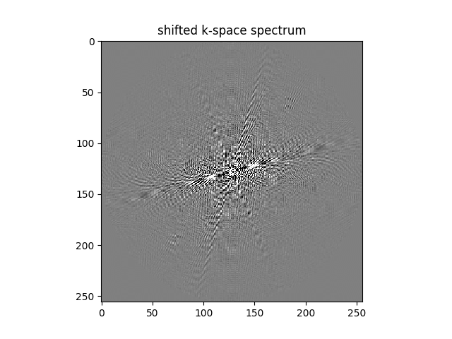
Fig. 8 The spectrum of the restored image solved by cg.